Tutorial 1

Preliminaries

For this tutorial:

The data can be found here fluidmechanics_data.mat
The configuration file here input_tutorial1.yaml
The complete Python script here tutorial1.py

Description

In this tutorial we explore a small dataset provided with this package that contains the flow exiting a nozzle (also referred to as a jet) from Bres et al.. The data is the symmetric component of a three-dimensional jet, and therefore itself two-dimensional. It is provided in equally-spaced cylindrical coordinates (r,x).

Starting from this dataset, we show how to:

load the required libraries, data and parameters,
extract the SPOD modes,
compute the time coefficients, by projecting the data on the SPOD basis built by gathering the modes, and
reconstruct the high-dimensional data from the coefficients

In detail, the dataset consists of 1000 flow realizations which represent the pressure field at different time instants. The time step is 0.01 seconds.


Animation of the data used in this tutorial.

1. Load libraries, data and parameters

The dataset is part of the data used for the regression tests that come with this library and is stored into tests/data/fluidmechanics_data.mat. The first step to analyze this dataset is to import the required libraries, including the custom libraries

import numpy as np
from pyspod.spod.standard  import Standard  as spod_standard
from pyspod.spod.streaming import Streaming as spod_streaming

The second step consists of loading the data from the fluidmechanics_data.mat. To this end, we provide a reader that accept .nc, .npy, and .mat formats.

data_file = os.path.join(CFD,'./data', 'fluidmechanics_data.mat')
data_dict = utils_io.read_data(data_file=data_file)
data = data_dict['p'].T
dt = data_dict['dt'][0,0]
nt = data.shape[0]
x1 = data_dict['r'].T; x1 = x1[:,0]
x2 = data_dict['x'].T; x2 = x2[0,:]

The third step is to read the parameters, that should be provided in Python dictionary format. We conveniently provide a yaml configuration file reader tailored to PySPOD.

config_file = os.path.join(CFD, 'data', 'input_tutorial1.yaml')
params = utils_io.read_config(config_file)

We can override some parameters in the dictionary in case it is needed. In this tutorial, we want to set the time step from the data we loaded, so, we write

params['time_step'] = dt

where dt has been previously defined when loadin the data.

2. Compute SPOD modes and visualize useful quantities

2.1 Computation SPOD modes

We can now run the PySPOD library on our data to obtain the SPOD modes. This is done by initializing the class and running the fit method:

standard = spod_standard(params=params, comm=comm)
spod = standard.fit(data_list=data)

where params, comm, and data have all been defined above. The spod_standard class implements the SPOD batch algorithm, as described in About. We can alternatively choose the streaming algorithm, by writing

streaming = spod_streaming(params=params, comm=comm)
spod = streaming.fit(data_list=data)

After computing the SPOD modes, we can check their orthogonality, to make sure that the run went well

results_dir = spod.savedir_sim
flag, ortho = utils_spod.check_orthogonality(
    results_dir=results_dir, mode_idx1=[1],
    mode_idx2=[0], freq_idx=[5], dtype='double',
    comm=comm)

where we retrieved the path where the SPOD modes were saved, using results_dir = spod.savedir_sim. The above orthogonality check, for the modes considered, should return: flag = True, and ortho < 1e-15 (i.e., the mode 1 and mode 0 for frequency id 5, are orthogonal as expected).

2.2 Visualization

PySPOD comes with some useful postprocessing routines. These can for instance visualize:

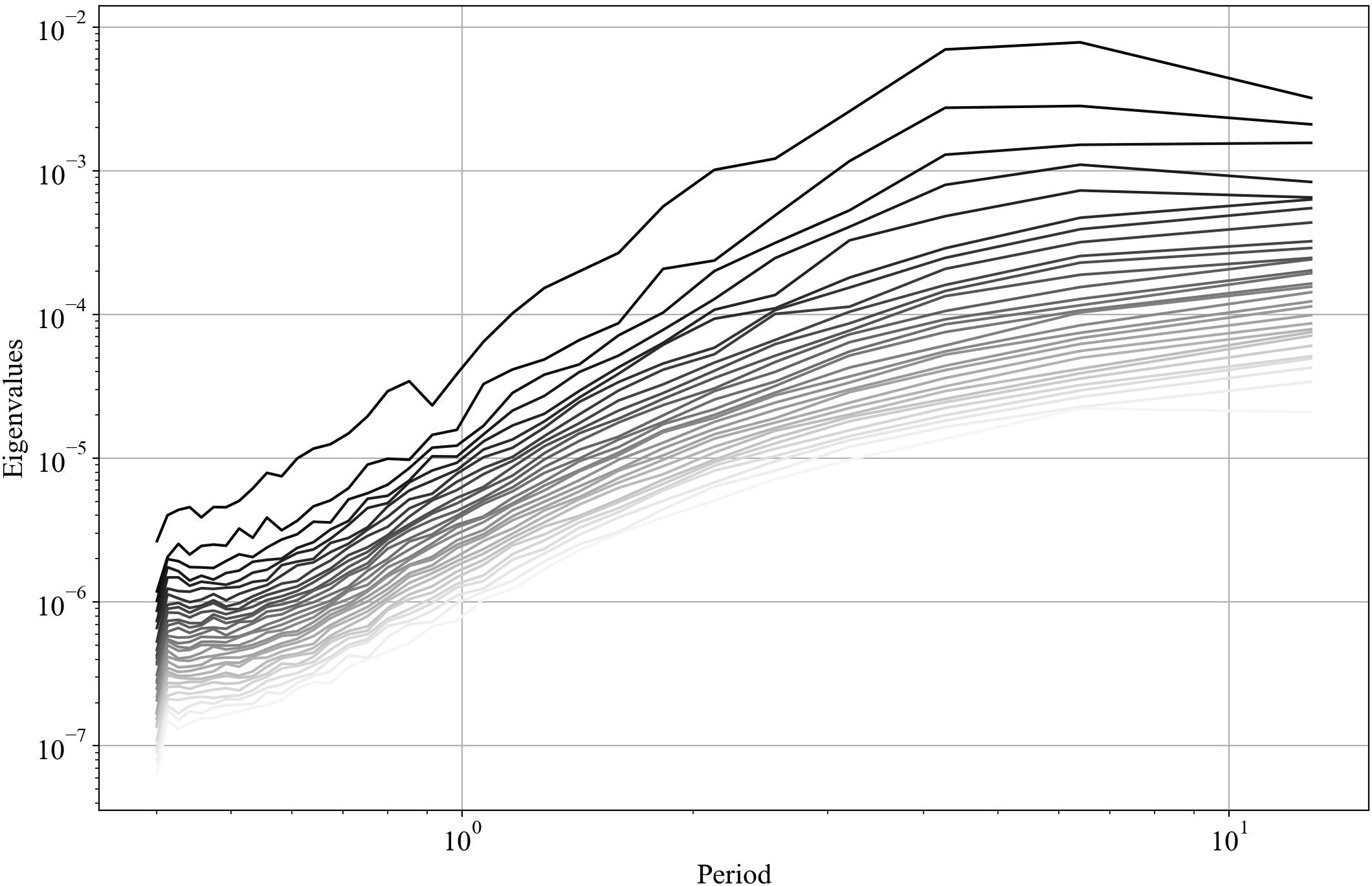
the eigenvalues, and the eigenvalues vs period (and frequency),

if rank == 0:
  spod.plot_eigs(filename='eigs.jpg')
  spod.plot_eigs_vs_period(filename='eigs_period.jpg')


Eigenvalues	Eigenvalues vs period

the SPOD modes for different frequencies

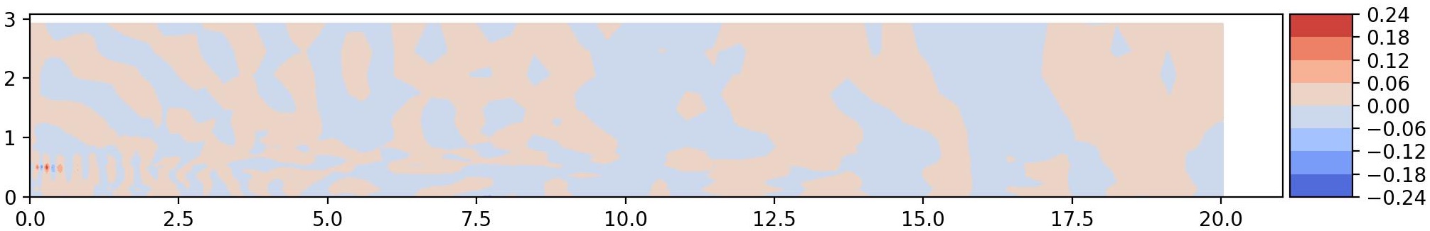
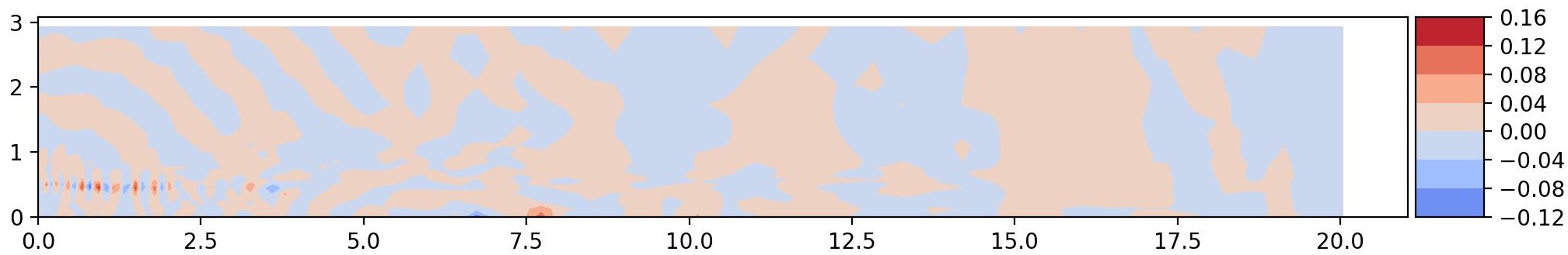
## identify frequency of interest
T1 = 0.9; T2 = 4
f1, f1_idx = spod.find_nearest_freq(freq_req=1/T1, freq=spod.freq)
f2, f2_idx = spod.find_nearest_freq(freq_req=1/T2, freq=spod.freq)
if rank == 0:
  ## plot 2d modes at frequency of interest
  spod.plot_2d_modes_at_frequency(freq_req=f1, freq=spod.freq,
      modes_idx=[0,1,2], x1=x2, x2=x1, equal_axes=True,
      filename='modes_f1.jpg')

  ## plot 2d modes at frequency of interest
  spod.plot_2d_modes_at_frequency(freq_req=f2, freq=spod.freq,
      modes_idx=[0,1,2], x1=x2, x2=x1, equal_axes=True,
      filename='modes_f2.jpg')


Mode 0, Period = 0.85	Mode 1, Period = 0.85


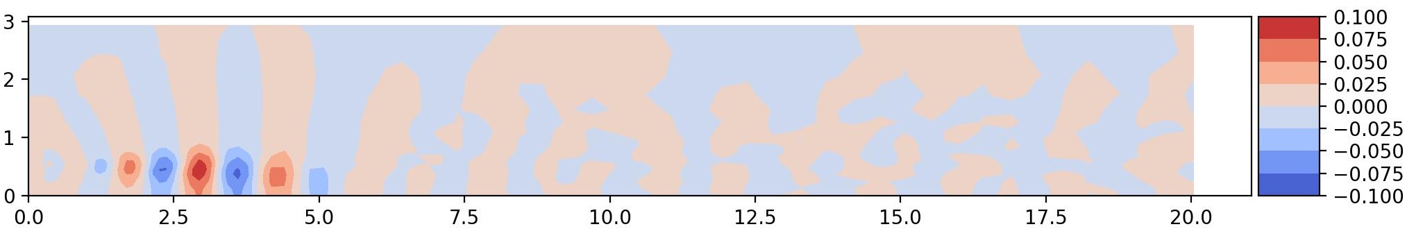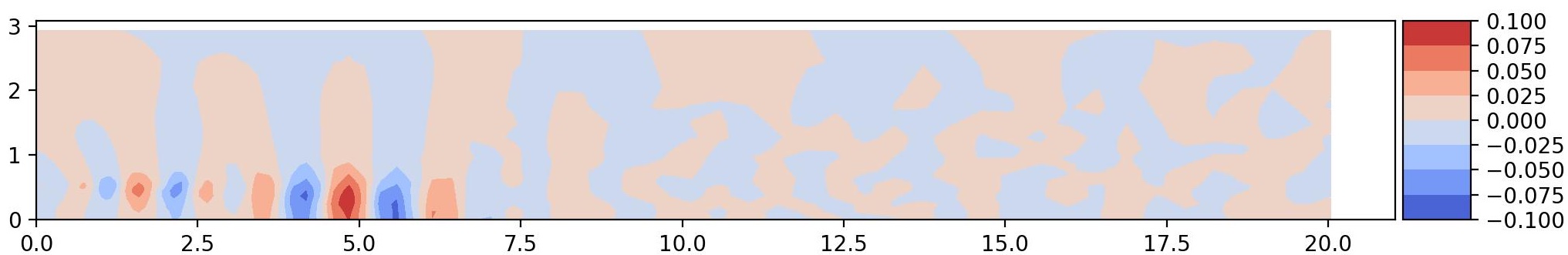Mode 0, Period = 4	Mode 1, Period = 4

Note that we are performing these visualization steps in rank = 0, only.

3. Approximate time-dependent coefficients via oblique projection

We can then compute the time coefficients and reconstruct the high-dimensional solution using a reduced set of them, and the associated SPOD modes. The method used here is the one referred to as oblique projection by Nekkanti and Schmidt.

These two steps can be achieved as follows

file_coeffs, coeffs_dir = utils_spod.compute_coeffs(
    data=data, results_dir=results_dir, comm=comm)

where we retrieved the path where the SPOD modes were saved, using the previously ran command results_dir = spod.savedir_sim.

We can visualize them as follows

coeffs = np.load(file_coeffs)
post.plot_coeffs(coeffs, coeffs_idx=[0,1], path=results_dir,
    filename='coeffs.jpg')


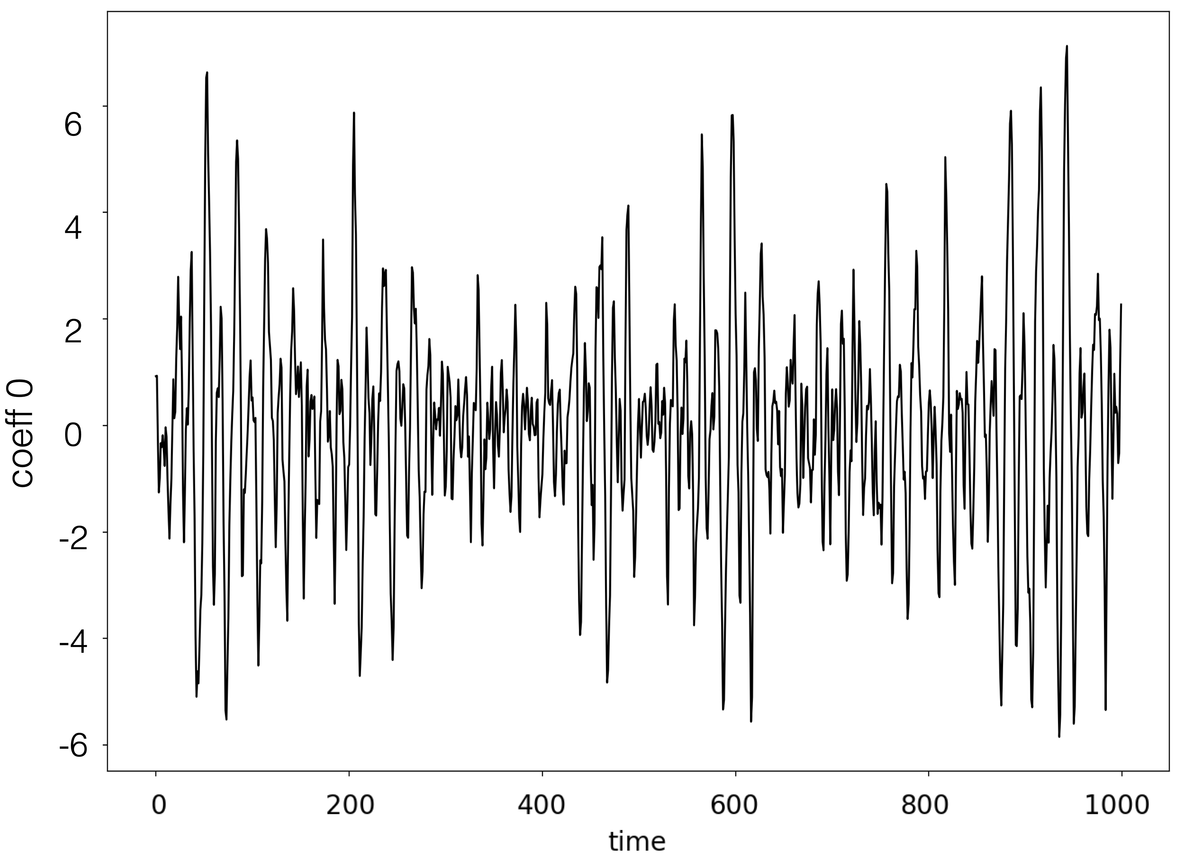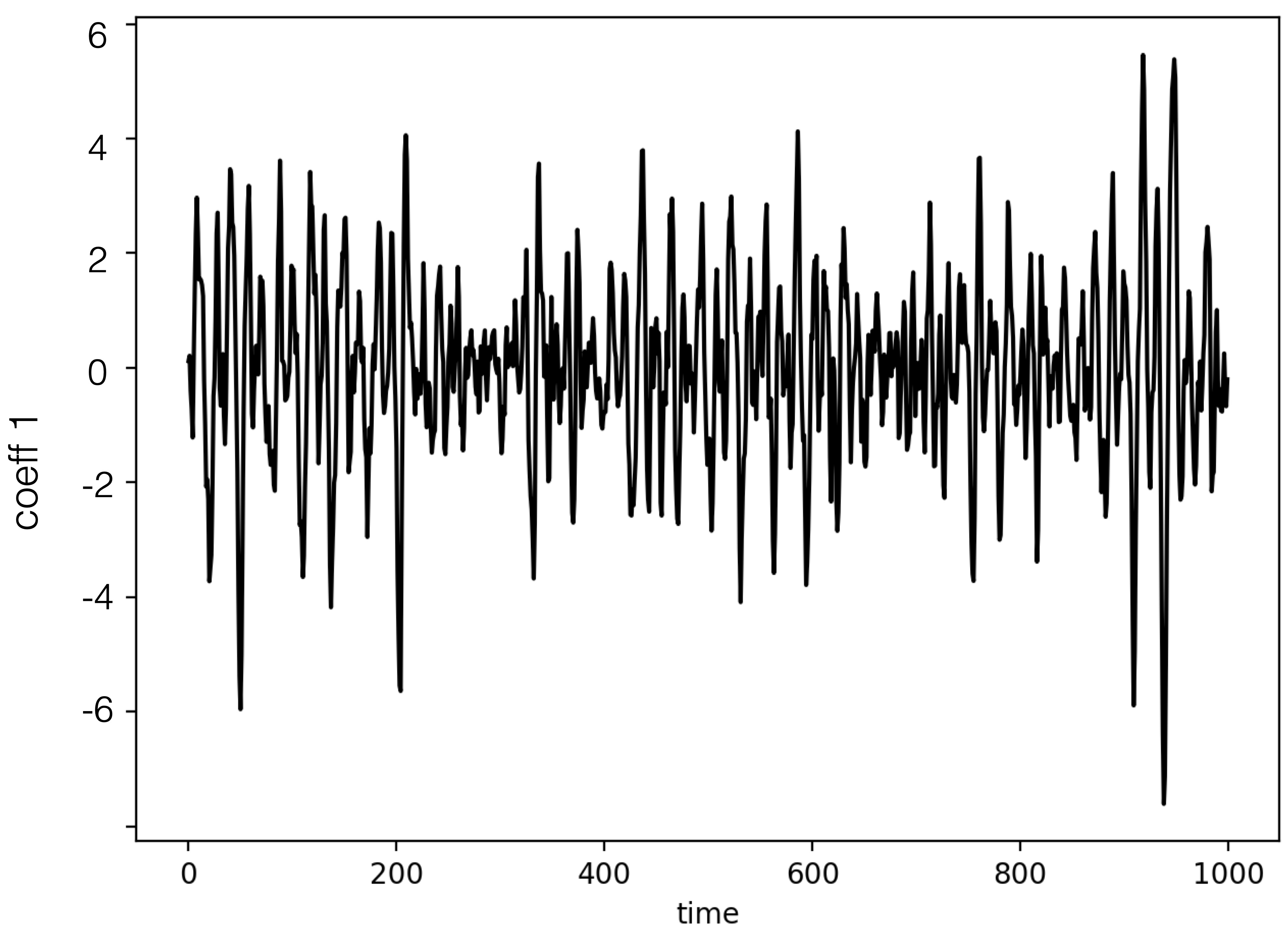Coefficient 0	Coefficient 1

4. Reconstruct high-dimensional data

We can finally reconstruct the high-dimensional data using the SPOD modes and time coefficients computed in the previous steps. This can be achieved as follows

file_dynamics, coeffs_dir = utils_spod.compute_reconstruction(
    coeffs_dir=coeffs_dir, time_idx='all', comm=comm)

where we retrieved the path where the SPOD coefficients were saved, using coeffs_dir, that was given when computing the coefficient in the previous step.

The argument time_idx can be chosen to reconstruct only some time snapshots (by specifying a list of ids) instead of the entire solution.

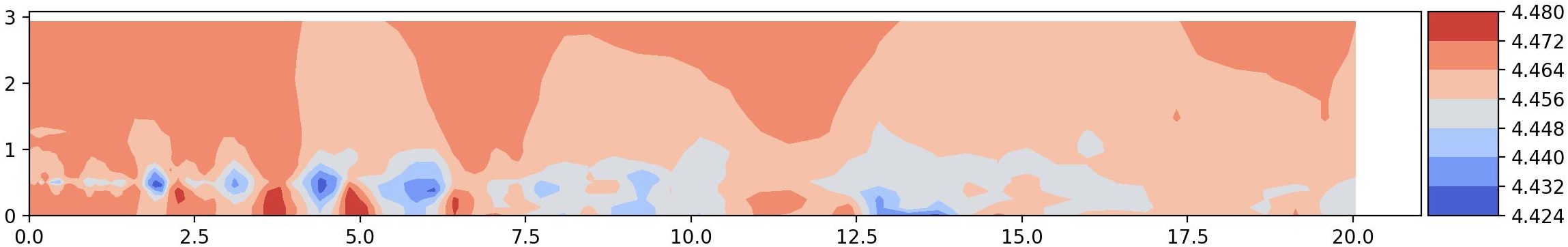
Also in this case, we can visualize the reconstructed solution, and compare it against the original data. Below, we compare time ids 0, and 10:

## plot reconstruction
recons = np.load(file_dynamics)
post.plot_2d_data(recons, time_idx=[0,10], filename='recons.jpg',
    path=results_dir, x1=x2, x2=x1, equal_axes=True)

## plot data
data = spod.get_data(data)
post.plot_2d_data(data, time_idx=[0,10], filename='data.jpg',
    path=results_dir, x1=x2, x2=x1, equal_axes=True)



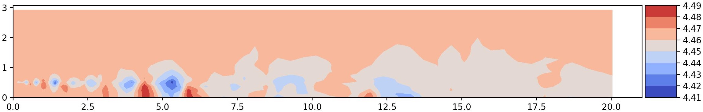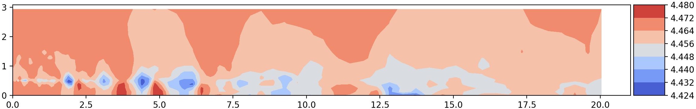Time id 0: true data (top); reconstructed data (bottom)	Time id 1: true data (top); reconstructed data (bottom)**

Go to the Home Page