Tutorial 2

Preliminaries

For this tutorial:

The data can be found here era_interim_data.nc
The configuration file here input_tutorial2.yaml
The complete Python script here tutorial2.py

Description

In this tutorial we explore a reanalysis dataset provided with this package that contains total precipitation data over Earth. The data is two-dimensional on a longitude-latitude grid, and is part of the ERA Interim dataset provided by ECMWF (please, refer to ERA Interim for more details). The dataset was reduced to include only the period 2008-2017, on a longitude-latitude grid that was also downsampled by a factor 5.

Starting from this dataset, we show how to:

load the required libraries, data and parameters,
extract the SPOD modes,
compute the time coefficients, by projecting the data on the SPOD basis built by gathering the modes, and
reconstruct the high-dimensional data from the coefficients

In detail, the dataset consists of 7305 time snapshots which represent the total precipitation field at different time instants. The time step is 12 hours, and it is sampled every day, in the period 2008 to 2017 at 03:00, and 15:00.


Animation of the total precipitation field data used in this tutorial.

1. Load libraries, data and parameters

The dataset is part of the data used for the regression tests that come with this library and is stored into tests/data/era_interim_data.nc. The first step to analyze this dataset is to import the required libraries, including the custom libraries

import numpy as np
from pyspod.spod.standard  import Standard  as spod_standard
from pyspod.spod.streaming import Streaming as spod_streaming

The second step consists of loading the data from the era_interim_data.nc. To this end, we provide a reader that accept .nc, .npy, and .mat formats.

data_file = os.path.join(CFD, './data/', 'era_interim_data.nc')
ds = utils_io.read_data(data_file=data_file)
t = np.array(ds['time'])
x1 = np.array(ds['longitude']) - 180
x2 = np.array(ds['latitude'])
data = ds['tp']
nt = len(t)

The third step is to read the parameters, that should be provided in Python dictionary format. We conveniently provide a yaml configuration file reader tailored to PySPOD.

config_file = os.path.join(CFD, 'data', 'input_tutorial2.yaml')
params = utils_io.read_config(config_file)

Given that the grid points of our data are not equi-spaced, we need to compute the weights. We provide a conveniently pre-implemented version of 2D trapezoidal weights that can be used for this case, and that can be used as follows:

## set weights
weights = utils_weights.geo_trapz_2D(
    x1_dim=x2.shape[0], x2_dim=x1.shape[0],
    n_vars=params['n_variables'])

2. Compute SPOD modes and visualize useful quantities

2.1 Computation SPOD modes

We can now run the PySPOD library on our data to obtain the SPOD modes. This is done by initializing the class and running the fit method:

standard = spod_standard (params=params, weights=weights, comm=comm)
spod = standard.fit(data_list=data)

where params, comm, weights and data, have all been defined above. The spod_standard class implements the SPOD batch algorithm, as described in About. We can alternatively choose the streaming algorithm, by writing

streaming = spod_streaming(params=params, weights=weights, comm=comm)
spod = streaming.fit(data=data, nt=nt)

After computing the SPOD modes, we can check their orthogonality, to make sure that the run went well

results_dir = spod.savedir_sim
flag, ortho = utils_spod.check_orthogonality(
    results_dir=results_dir, mode_idx1=[1],
    mode_idx2=[0], freq_idx=[5], dtype='double',
    comm=comm)

where we retrieved the path where the SPOD modes were saved, using results_dir = spod.savedir_sim. The above orthogonality check, for the modes considered, should return: flag = True, and ortho < 1e-15 (i.e., the mode 1 and mode 0 for frequency id 5, are orthogonal as expected).

2.2 Visualization

PySPOD comes with some useful postprocessing routines. These can for instance visualize:

the eigenvalues, and the eigenvalues vs period (and frequency),

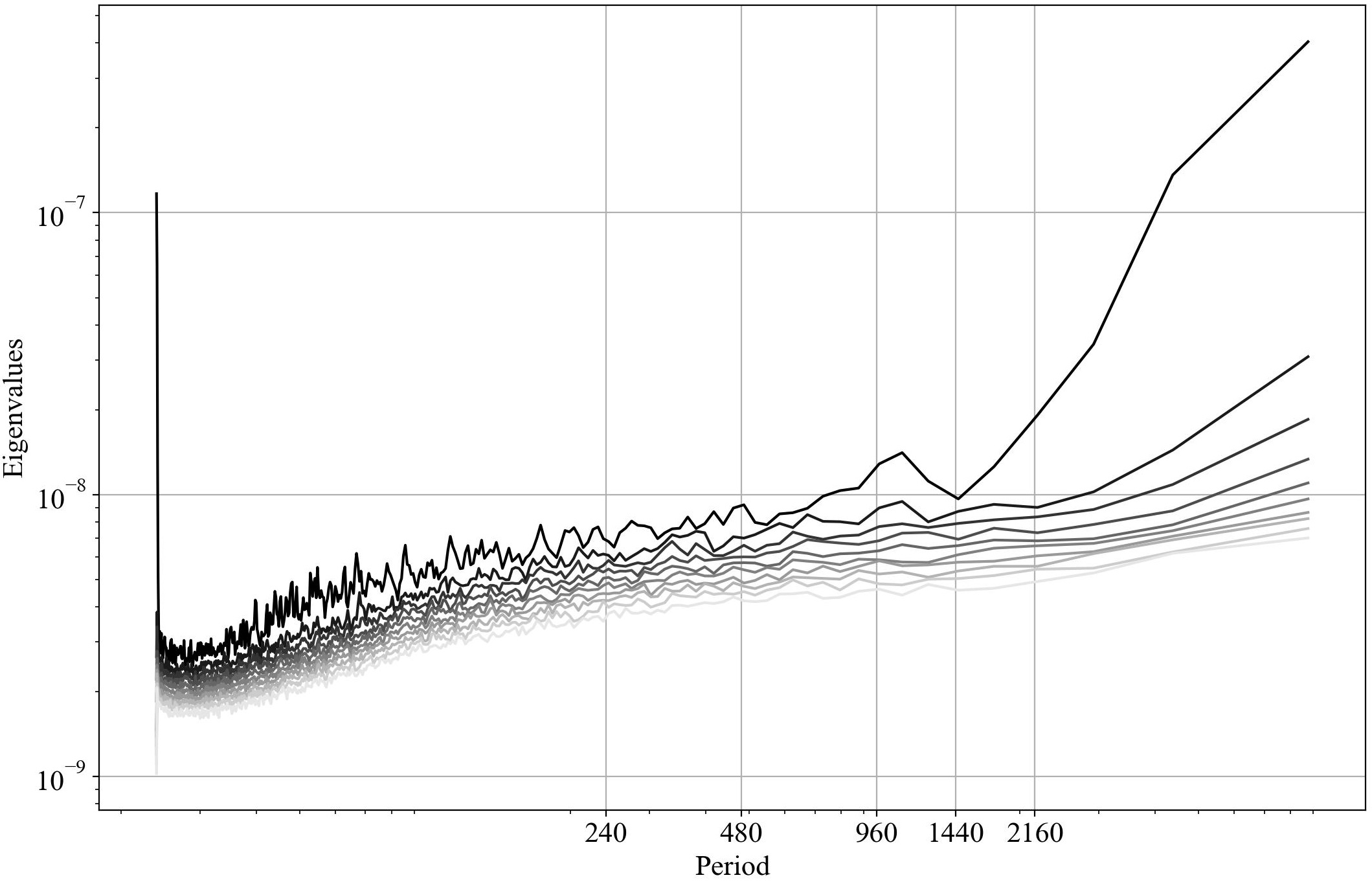
if rank == 0:
  spod.plot_eigs(filename='eigs.jpg')
  spod.plot_eigs_vs_period(filename='eigs_period.jpg')


Eigenvalues	Eigenvalues vs period

In the right figure, we can see that there is a peak at around 40 days (960 hours). This is approximately the average period of the Madden-Julian Oscillation, or MJO. The MJO is an intraseasonal phenomenon that characterizes the tropical atmosphere. Its characteristic period varies between 30 and 90 days and it is due to a coupling between large-scale atmospheric circulation and deep convection. This pattern slowly propagates eastward with a speed of 4 to 8 $ms^{−1}$. MJO is a rather irregular phenomenon and this implies that the MJO can be seen at a large-scale level as a mix of multiple high-frequency, small-scale convective phenomena.

the SPOD modes for different frequencies

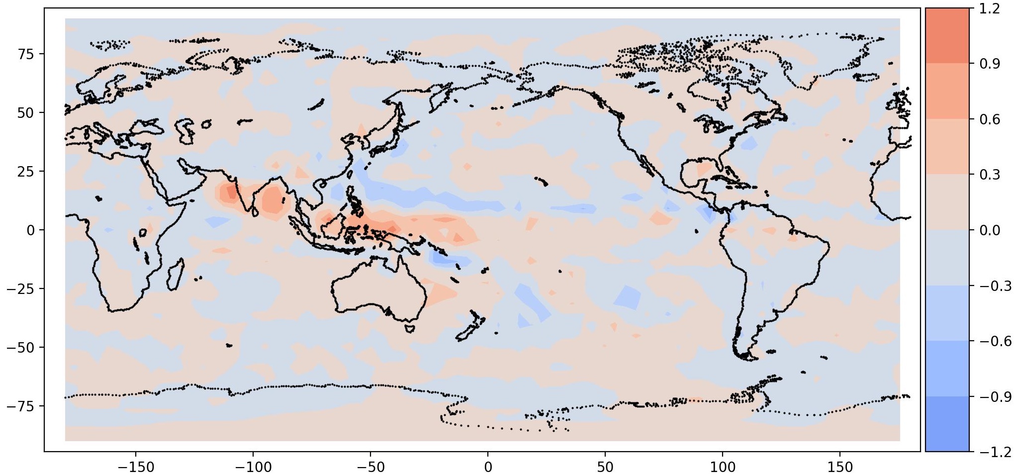
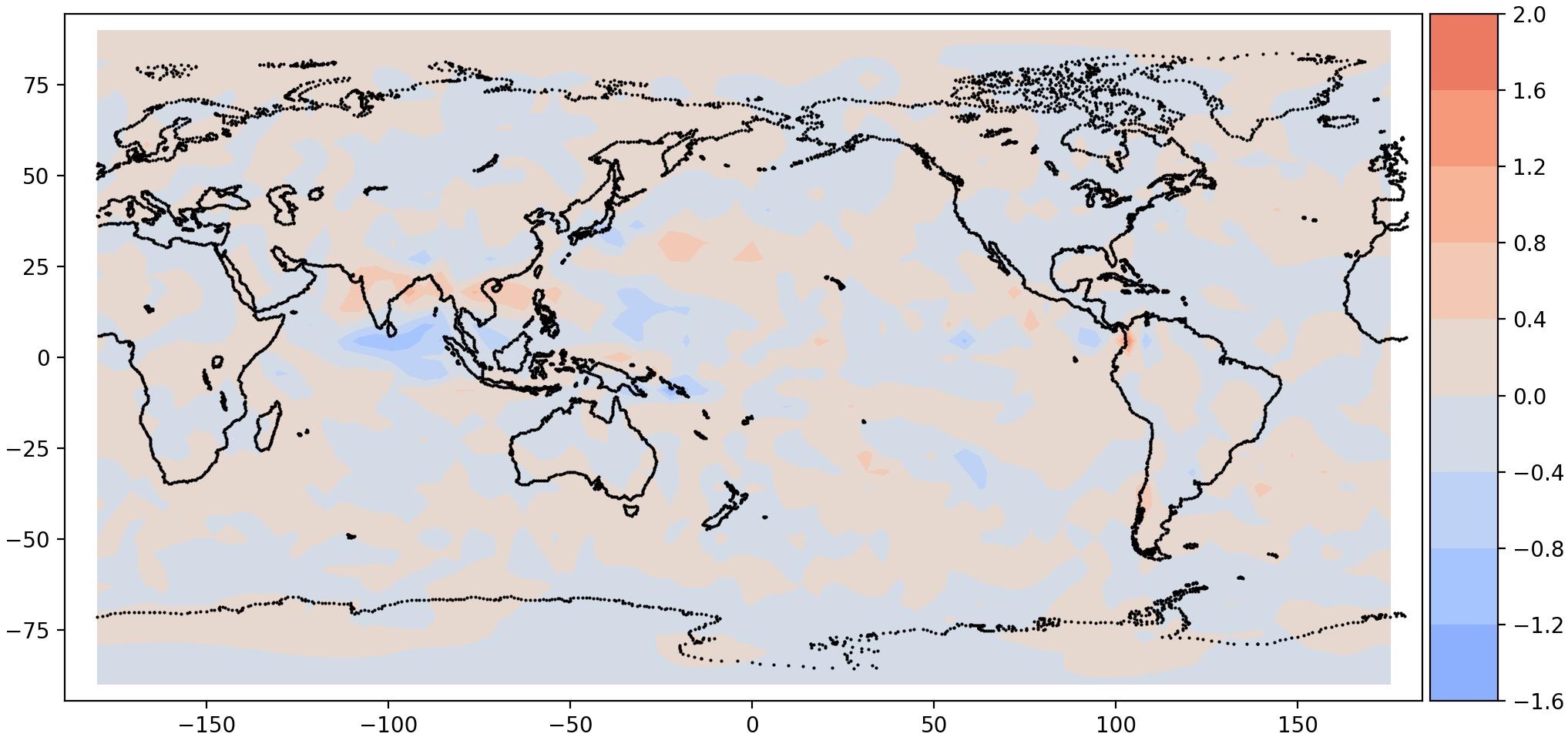
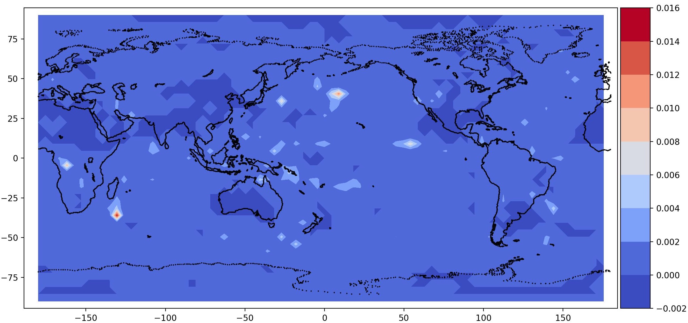
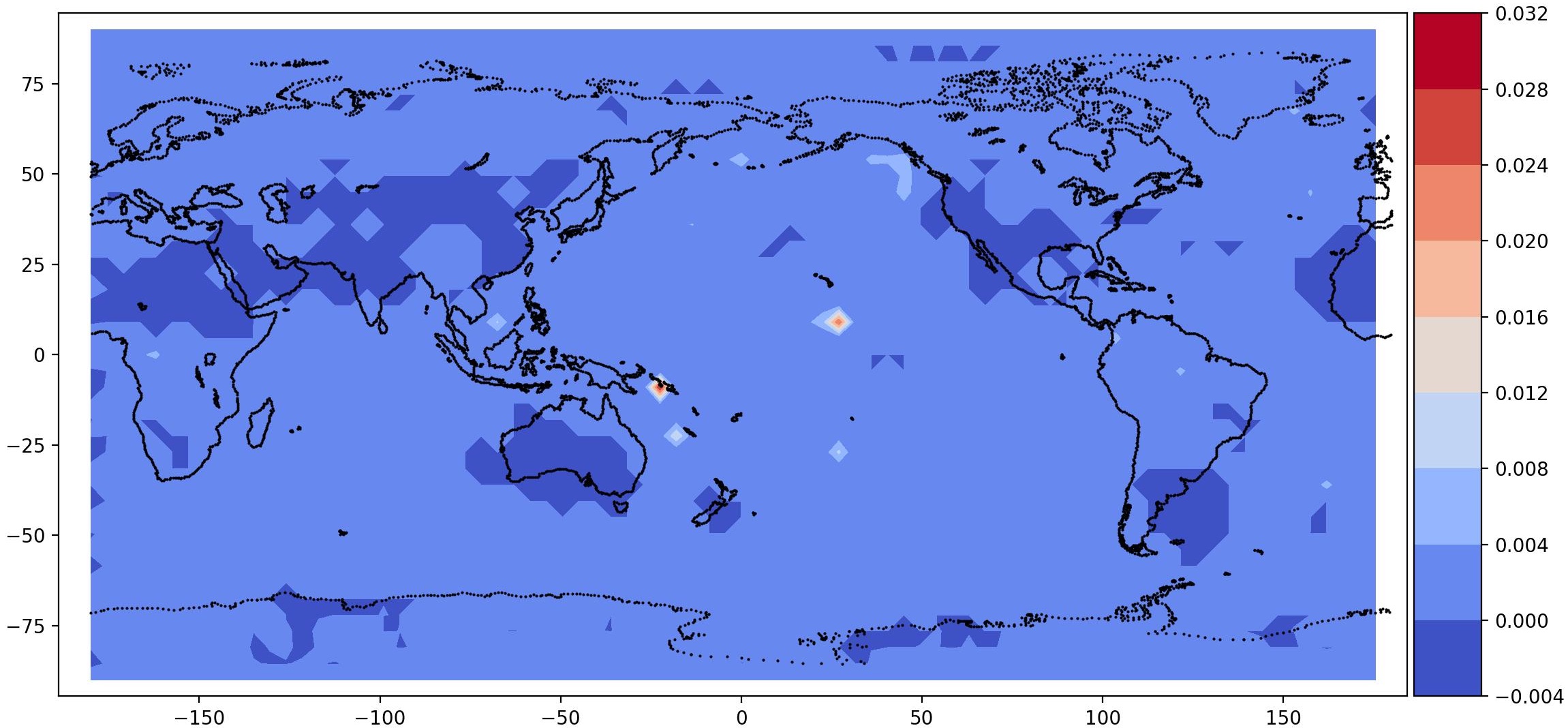
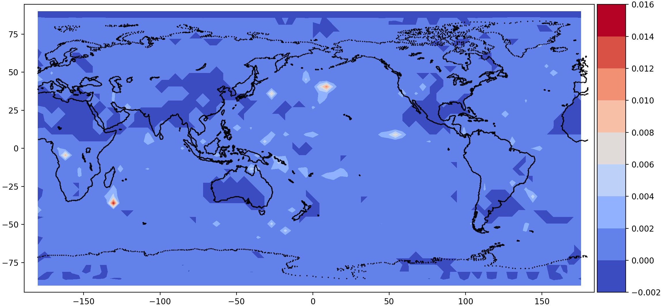
## identify frequency of interest
T1 = 960; T2 = 1008
f1, f1_idx = spod.find_nearest_freq(freq_req=1/T1, freq=spod.freq)
f2, f2_idx = spod.find_nearest_freq(freq_req=1/T2, freq=spod.freq)
if rank == 0:
  ## plot 2d modes at frequency of interest
  spod.plot_2d_modes_at_frequency(freq_req=f1, freq=spod.freq,
      modes_idx=[0,1,2], x1=x2, x2=x1, equal_axes=True,
      filename='modes_f1.jpg')

  ## plot 2d modes at frequency of interest
  spod.plot_2d_modes_at_frequency(freq_req=f2, freq=spod.freq,
      modes_idx=[0,1,2], x1=x2, x2=x1, equal_axes=True,
      filename='modes_f2.jpg')


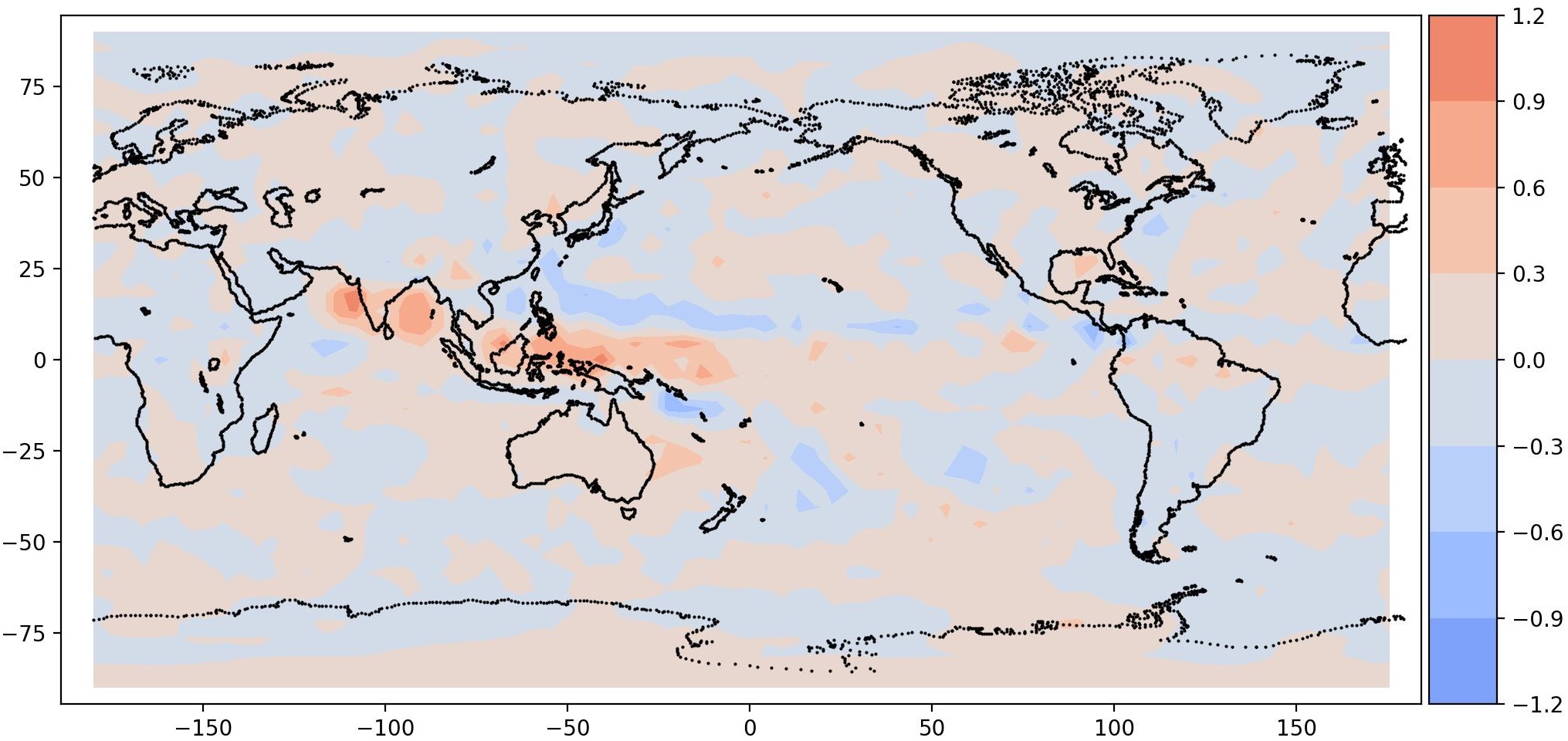
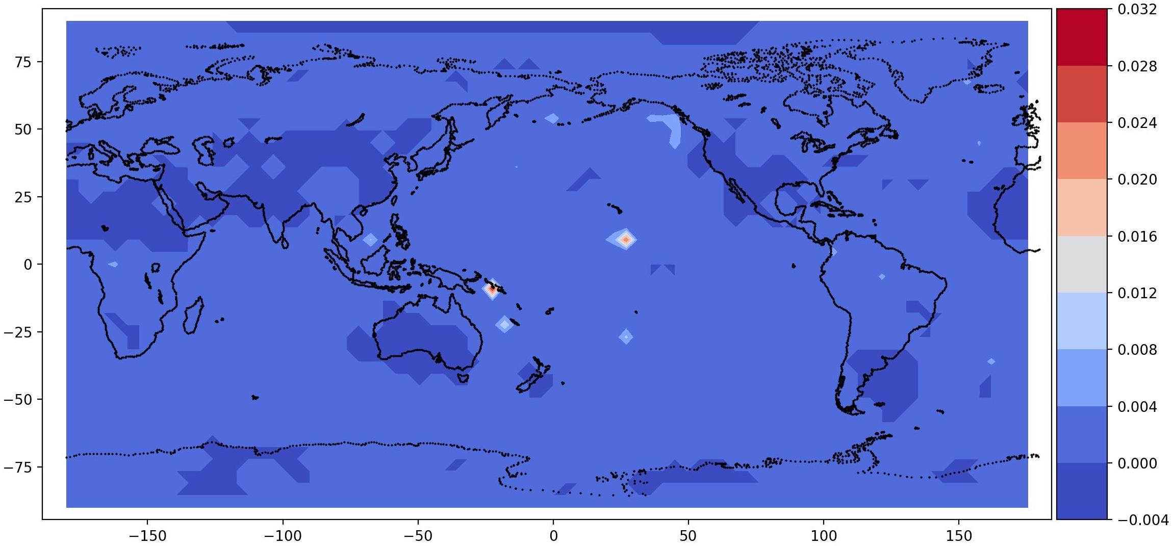
Mode 0, Period = 960	Mode 1, Period = 960


Mode 0, Period = 1008	Mode 1, Period = 1008

It is interesting to note a total precipitation pattern in South East Asia, as expected. This is the signature of MJO. It should be noted that the data is very coarse, hence the resolution is also coarse.

Note that we are performing these visualization steps in rank = 0, only.

3. Compute time coefficients

We can then compute the time coefficients and reconstruct the high-dimensional solution using a reduced set of them, and the associated SPOD modes.

These two steps can be achieved as follows

file_coeffs, coeffs_dir = utils_spod.compute_coeffs(
    data=data, results_dir=results_dir, comm=comm)

where we retrieved the path where the SPOD modes were saved, using the previously ran command results_dir = spod.savedir_sim.

We can visualize them as follows

coeffs = np.load(file_coeffs)
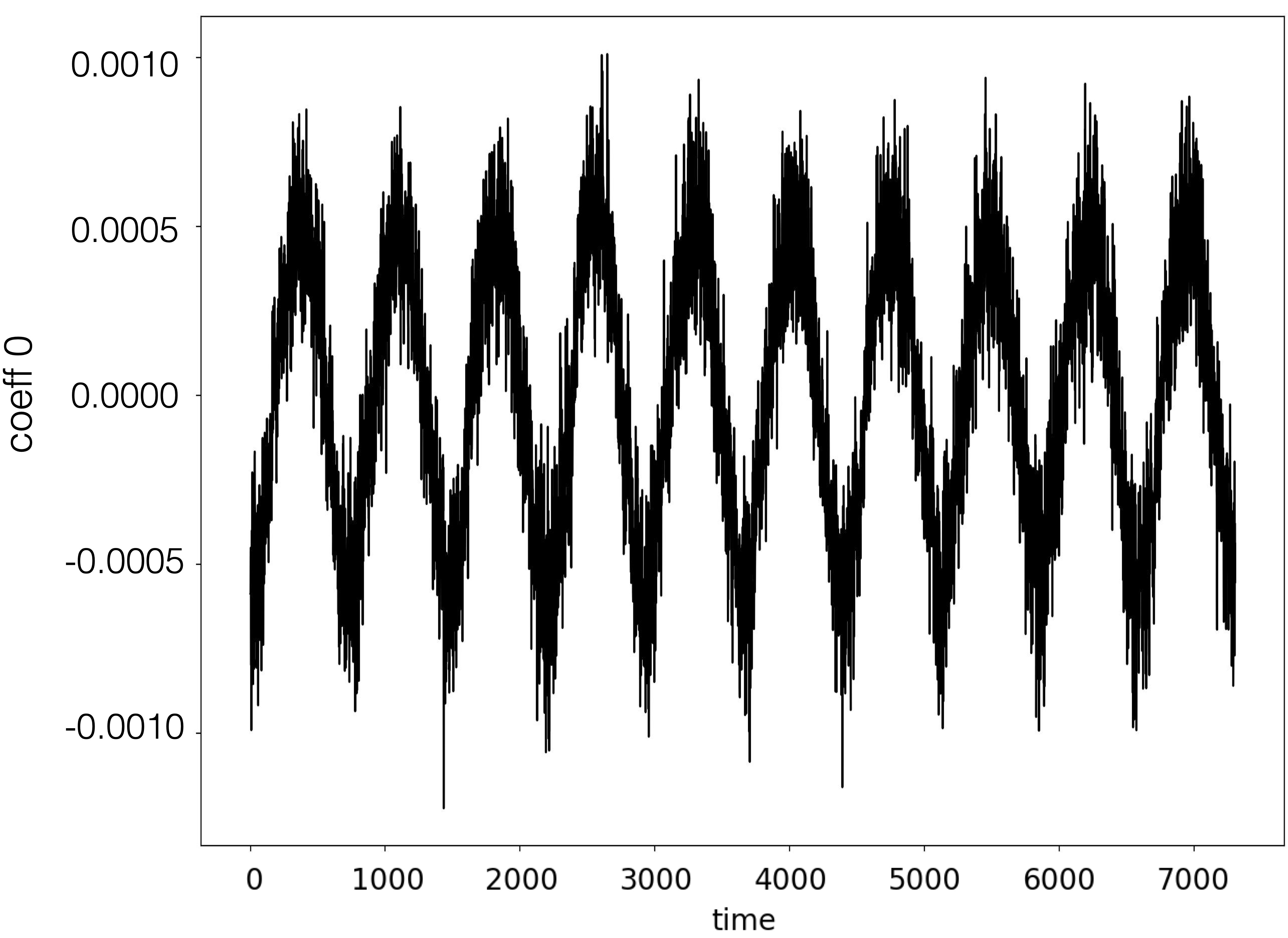
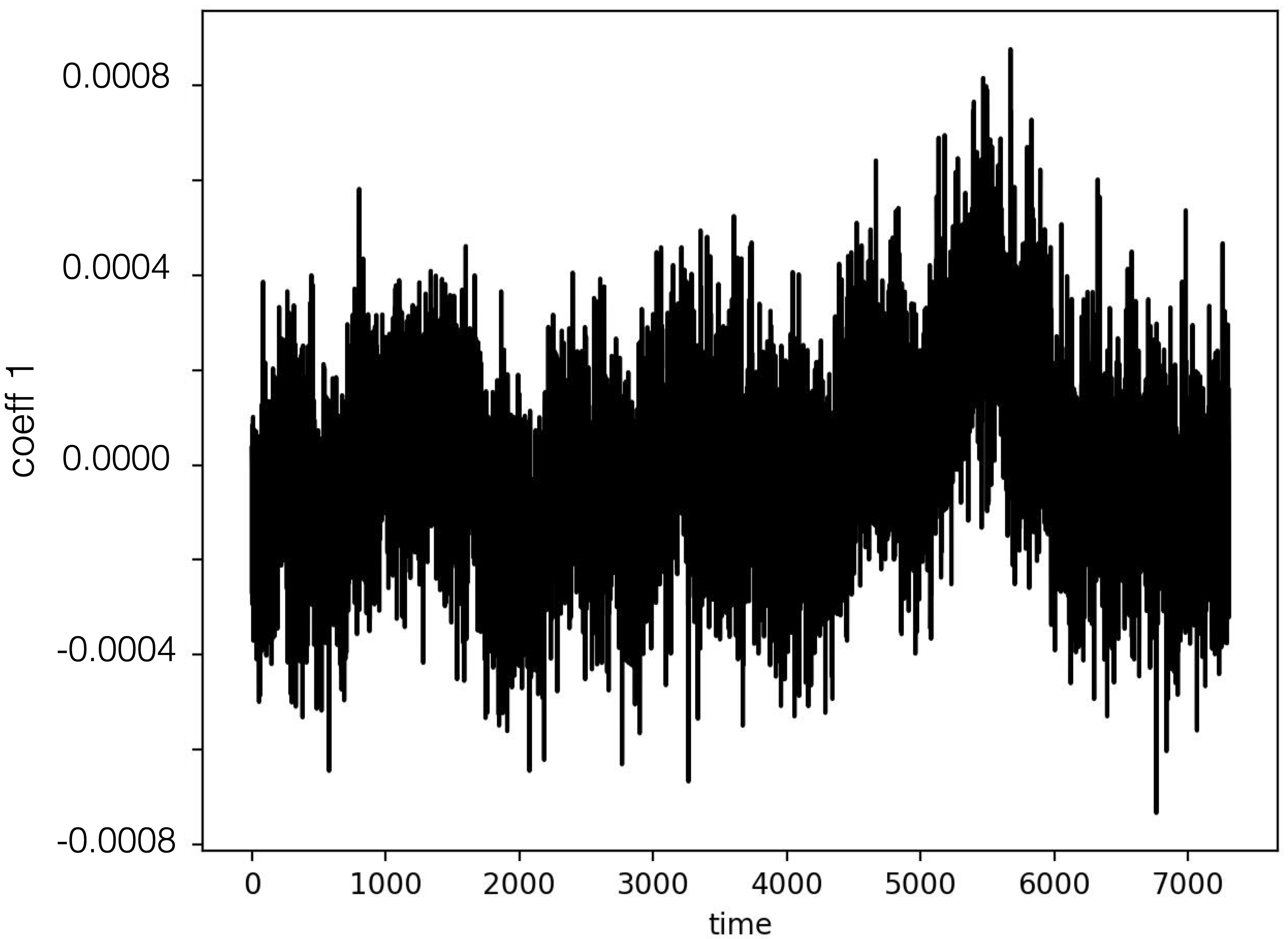
post.plot_coeffs(coeffs, coeffs_idx=[0,1], path=results_dir,
    filename='coeffs.jpg')


Coefficient 0	Coefficient 1

Note that this step may require some time.

4. Reconstruct high-dimensional data

We can finally reconstruct the high-dimensional data using the SPOD modes and time coefficients computed in the previous steps. This can be achieved as follows

file_dynamics, coeffs_dir = utils_spod.compute_reconstruction(
    coeffs_dir=coeffs_dir, time_idx='all', comm=comm)

where we retrieved the path where the SPOD coefficients were saved, using coeffs_dir, that was given when computing the coefficient in the previous step.

The argument time_idx can be chosen to reconstruct only some time snapshots (by specifying a list of ids) instead of the entire solution.

Also in this case, we can visualize the reconstructed solution, and compare it against the original data. Below, we compare time ids 0, and 10:

## plot reconstruction
recons = np.load(file_dynamics)
post.plot_2d_data(recons, time_idx=[0,10], filename='recons.jpg',
    path=results_dir, x1=x2, x2=x1, equal_axes=True)

## plot data
data = spod.get_data(data)
post.plot_2d_data(data, time_idx=[0,10], filename='data.jpg',
    path=results_dir, x1=x2, x2=x1, equal_axes=True)



Time id 0, true data (top); reconstructed data (bottom)	Time id 1, true data (top); reconstructed data (bottom)